An Intelligence Device Used to Detect and Autofocus 3D Microstructures from Ordinary Optical Microscope

Why NVIDIA Jetson TX2?

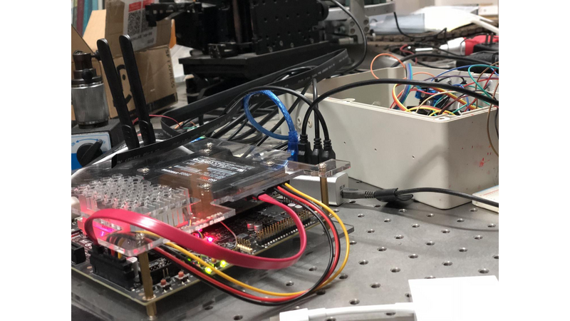
Jetson TX2 is the fastest, most power-efficient embedded AI computing device. Its Power consumption is 7.5-watt. It's built around an NVIDIA Pascal-family GPU and loaded with 8 GB of memory and 59.7 GB/s of memory bandwidth. As its internal storage is a bit small and we need to take a big data we added 256 GB SSD.

Modification of microscope

The conventional method of adjusting the ordinary optical microscope to be suitable for stepper and servo motors in the process of finding a clear sample image, as well as autofocusing, can be discussed as follows.

Step 1: Adjust the x-y-z hand wheel of the carrier so that the object is aligned to the objective lens, making it appear in the center of the field of vision.

Step 2: Adjust the coarse coke screw knob to find the fuzzy image.

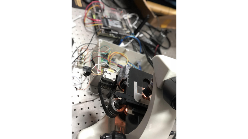
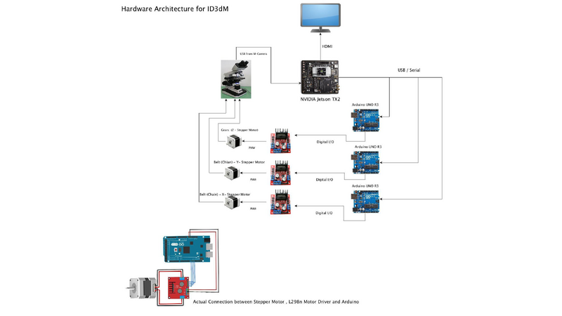
Step 3: Adjust the fine focusing screw to find the clear image. We've modified the microscope to automate this process. Install two sets of pulleys on the X adjustment knob of the carrier platform and the Y adjusting knob of the carrier platform respectively. Similarly, a set of pulleys is also fixed on the coarse coke screw knob. Connect the camera with an electronic eyepiece to observe the image in real time.

Belt driving principle

The belt drive is composed of an active wheel, a moving wheel, and a conveyor belt. Because we want to achieve synchronous transmission, we need to use meshing belt transmission, also called synchronous belt drive. This kind of belt transmission depends on the motion and power of the meshing between the isometric lateral teeth with the inner circumference and the corresponding cogging of the pulley. One side of the wheel is connected to stepper motor X to control X knob and another side is connected to the knob. This process is repeated for knob Y as well.

Finding the Sample

Finding the sample is consisting of two mainly organized algorithms. One is dealing with the mechanical part which is controlling the motors where the motors controlled the knobs and another one is AI which is a set of Machine learning and computer vision which control the finding and autofocusing on the sample.

The Mechanical Method

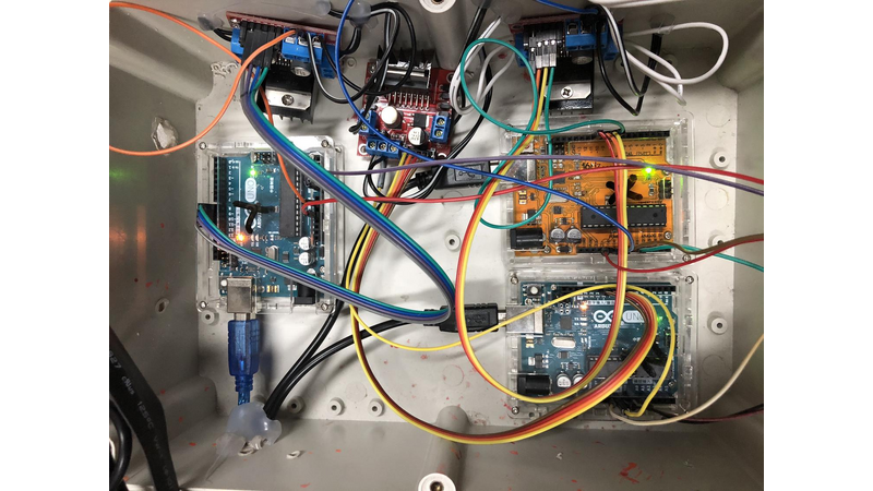
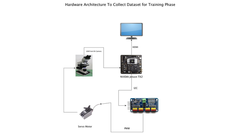
By using three stepper motors to control X-Y-Z position knobs and one servo motor(to take dataset for training phase) to control the focusing knob, all motors connected to their equivalent Arduinos using PWM digital output and Arduinos connected to NVIDIA Jetson TX2 using a Serial USB cable. From starting point (X0, Y0, Z0) and ending point (Xn, Yn, Zn) on the microscope slide the sample finding mechanism is continuous in a given Z-direction where there will be an increment in X till it reaches Xn Then Y, after Y increased in one value X, starts from X0 to Xn when Y reach Yn Z will increase by one value. A Python script backend with Computer Vision and Machine Learning will see each pixel and control the movement of the motors and to find any samples in detected XY area if the sample is matched with our sample it will proceed to the next step else it will continue the process until the ending point (Xn, Yn, Zn) of the microscope slide.

The AI algorithm

From finding the microstructures, matching the sample from a microscope slide to plotting the equivalent 3D model we use AI. The whole programming language is written using Python and backend with C++. OpenCV, Tensorflow, Keras, Scikit and MatPlot Lib are widely used libraries. We have different scripts for a different purpose. In the following description, we will discuss depending on their features and uses.

Machine Learning

Below training phase, we need to collect dataset and labeling them, then train our model.

the second one is using our trained models to find the sample.

The third one is matching the sample to know what kind of Sample it is.

The fourth one is detecting and separating the edges to make the 3D Model using Sketch.

Computer Vision

We use computer vision to separate total structures in the microscope slide during the autonomous mode. here we save each microstructures location in form os Numpy array. later on, we use these locations to match our sample and dirties.

Collecting the datasets:

Our input is a 2MP Microscope eyepiece camera which is connected to Jetson TX2 using USB. The script running on the NVIDIA Jetson TX2 is controlled the Arduino to control the servo motor and get a sequence of frames using the camera from the Microscope slide. We have collected around 5000 positive images using series frame recording. By rotating the servo motor in each angle, we can get a unique edge feature from the sample then we have saved each frame as a 640X480 AVI video file, this is helpful to not miss any frames and features with a mismatch of the speed of the rotation and recording rate. After saving the video we will extract the video as 640X480 images as JPG format. The servo controlling mechanism is, If the range of rotation of the servo motor is from 0 to 90 degrees, the height of the structure is given and range factor is calculated from the angle difference of the maximum angle. With each and given T (where T is the time used to rotate the servo motor by one angle) there will be X frames which will be saved as video files. After collecting our dataset image, we will put them in desired name folders where these folders name will be used as a label to train our model.

Training Our Model:We have designed different CNN (Convolutional Neural Network) models for this experiment, these are: Detecting the microstructures, to Identify the detected microstructures as our Sample and Not our Sample, identifying a type of the sample and autofocusing. For the identification of Sample and Not Sample training phase, we used the images containing our Sample gathered using Collecting the datasetsTechnique. And randomly 10000~ Images that do not contain our samples from our Lab database and internet. we used Tensorflow to train our model. Again, for detecting the Sample type we separated the images to their type, each of them has around 768 images. Each input image is represented as 64 x 64 grayscale image; we will simply resize our 640X480 images to 64X64 using OpenCV resize function or any other. These resized grayscale pixel intensities are unsigned integers, with the values of the pixels falling in the range [0, 255]. The reshaped layers change the shape of the data back into a 2D image for the convolutional layer. For convolutional layers, we need to select how many filters, and the size of the convolution area – too small or too large and we won't be able to obtain interesting features. The dropout layers' dropout rate is also important in order to balance learning and overfitting. All digits are placed on a black background with a light foreground (i.e. the sample itself) being white and various shades of gray. We have classified our dataset as 80% training and 20% test data. For sample and not sample classifier we have used 2 classes which is our sample and not sample our classes are similar to the label. Since this is a two-class classification problem we'll want to use binary cross-entropy as our loss function. By using Matplot-lib we have plotted the training loss, Val loss, train accuracy and value accuracy. The network trained for 80 epochs and we achieved high accuracy (~99.8%testing accuracy) and low loss that follows the training loss (Images is attached to the results). To identify the sample type as an experiment we used two types one is Six Edge Hexagon 3D microstructure and another one is four-edged Pyramid 3D microstructure. Here also we have used two classes one is for hexagon and for a pyramid. Our classes are similar to the label. Since this is a two-class classification problem we'll want to use binary cross-entropy as our loss function. By using Matplot lib we have plotted the training loss, Val loss, train accuracy and value accuracy. The network trained for 120 epochs and we achieved high accuracy (~98.5%testing accuracy).

Test Our Model

To test our models, we have to handle scaling our image to the range [0, 1], converting it to an array and adding an extra dimension. As we train/classify images in batches with CNN's. Adding an extra dimension to the array using Numpy arrays which allows our image to have the shape that we want. all our models succeeded in defining Samples and Non-Samples and what kind of sample it is, with almost ~0.01% loss.

Finding the Sample Autonomously Using CNN and CV

After we put our slide on the microscope the program will start to find the sample by controlling the stepper motors using Arduino. We use computer vision to differ the plane and any blobs. When there is a blob on the slide the program will save the location in terms of X, Y, Z. this is useful to know the blobs are either dirtied or real sample, to analyze this we use our trained model if the detected object is our sample we will save the location into Numpy arrays for later analysis.

Identifying the Sample

On the Previous step if we found the sample we will drive to the location from Numpy array and use the trained model to identify what kind of microstructure it is.

Autofocusing to the Widest Edge
Using computer vision and machine learning after detecting the sample we apply Gaussian filter then thresholding the image when we threshold the image we can easily see the image as 0 and 1 values again we apply canny edge detection for the widest edge will be clear enough from the model label we will approach the neighbor pixel either pull or drag to the existed pixel this will help us to get clear image of the sample in this process we use at least three images one as a master the remains are used for sliding the pixels.

Plot the 3D

Our input is flattening into Z-axis array and predict its exact location from 0 to N where n is the height of the sample. After we threshold our sample's current image using we can able to see each edge in the sample the applying canny edge we can see the current active edge the process continued by saving the edge using its edge number using Numpy and then by using Matplot lib 3D plot function we will plot a 3D image by constructing collected 2D edges on the Z direction from Numpy array. Our Matplot 3D axis's XYZ values are driven by the sample's XYZ value. Putting each edge on a given Z axis where Z is in ascending order with different images until we will get the final precise 3D model.

Contrast

For the four-pyramid specimen, we will scan it with sem. We compare the scanned four pyramid structure with the 3D microstructure obtained by our detection device and get the accuracy of the detection device.

The model simulation

We use a four-pyramid specimen to make a model. The four-pyramid model is the same as the specimen, with a length of 50 microns and a height of 37 microns. In the first step, the height gradient is set to 1 micron to obtain 35 pictures (there are 2 dropouts).

Application prospect

The device uses computer vision, machine learning, and computer programming to reduce the structure of some tiny 3D specimens. We can detect the products produced by femtosecond laser two-photon microfabrication. It can also detect a variety of micro products 3D microstructure in the future. And it can be applied to 3D printing inspection, 3D microprocessing, and testing industries.